Creating the Grid (Gridding)
Having the input branch completed and prior to obtaining the results crucial decisions have to be taken having major impact onto the precision of results and calculation time required to create them. The principle behind the calculation method of AnTherm lies in balancing the thermal characterisations of orthogonally subdivided regions. Each subdivision, or cell, is thus geometrically bound by orthogonal grid planes; these must be defined such that each resulting cell contains only a single building material. Thus, the resulting subdivisions need not to be identical with the input elements. The process of creating proper subdivisions is called "gridding".
Minimal Grid
 The coarsest grid structure which satisfies the requirement of homogeneous
cells is referred to as the minimal grid. This can be derived directly
from the geometric data (elements) of a
model. This minimal grid is generated fully
automatically without any further user intervention.
The coarsest grid structure which satisfies the requirement of homogeneous
cells is referred to as the minimal grid. This can be derived directly
from the geometric data (elements) of a
model. This minimal grid is generated fully
automatically without any further user intervention.
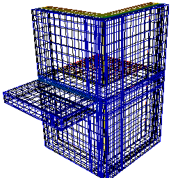
Fine Grid
Since a minimal grid is generally too coarse a subdivision to provide dependably accurate results by numerical methods, a further - finer - gridding of the model must be performed for calculation. AnTherm offers automatic method for generating such auxiliary grid planes. The minimal grid thus generated forms the basis for all further gridding, but it does not constitute a complete grid structure. A fine grid in some form must be generated and stored in a grid file before moving on in the calculation branch.The creation of a fine grid involves inserting additional grid planes. Such procedure might be very circuitous and tedious when done manually. Therefore AnTherm provides an automatic generation of the fine grid controlled with few parameters. The automated process ensures, that most critical regions (corners, edges, etc) will receive finest grid.
The fine-gridding defines the final set of cells (orthogonally subdivided regions) which shall then be balanced The number of such cell might be very large! Typical 2D calculation will result in 20.000-50.000 calls to solve with sufficient precision. 3D calculation will quickly grow to 1.000.000 cells and more!
The gridding (discretization) algorithm of AnTherm subdivides the component model under consideration into cells which will be thermally balanced thereafter. The calculation algorithm creates for each such cell the heat balance equation and then solves the system of such equations. The solution results describe temperature field with values in the middles of cells.
In the event that a minimal grid would suffice for calculation (e.g. for preliminary evaluation of a model), it can be re-generated as a fine grid based on the appropriate parameters.
Super Fine Grid (The "super" - refinement)
During the evaluation AnTherm will provide further refinement of this results. Here, by using heat balance and interpolation algorithms, AnTherm uses temperatures at cell centres to calculate temperatures at centres of cell edges, centres of cell surfaces and at each cell corner.
Considering places where temperatures will later be calculated (during the evaluation) not only middle points of each cell are of interest - middles of cell sides and cell edges and corners of each cell will be calculated too.
Such super-fine-gridding provides for the two dimensional calculation of 20.000 cell about 80.000 evaluated temperature points. Within a three dimensional case with a fine grid of 20.000 cells the evaluation will result in more than 160.000 temperature values. If the fine grid size is large - e.g. 1.000.000 cells for a 3D case - the number of calculated temperature points will grow to more than 8.000.000 possibly requiring longer calculation times during the evaluation. For that reason AnTherm will display a warning message when the number of cells within the fine-grid grows to higher value. In such case it is worth to consider, if, by adjusting some fine-grid parameters resulting in more coarse grid, sufficient precision can be reached faster also.
As the nice result of such refinement the provisioning of much higher number of node values is available for the evaluation, hence the evaluation can be much more precise thereafter - for the two dimensional case the number of temperature nodes is fourfold the original cell count and in three dimensional case it is eightfold! For example, the calculation with 1.000.000 (one million) balanced cells provides results of thermal balance equations at more than 8.000.000 (eight million) points! - and the operation is accomplished in surprisingly short computation time.
The most beneficial effect of this refinement can bee seen in that the temperatures at any material boundary can be provisioned that way! Material boundaries of special interest exist at the junction of different materials and, more importantly, at all surfaces of the component considered for analysis. Evaluating temperatures at component surfaces is essential to the evaluation and analysis of thermal bridges. Therefore the super refinement shall be seen as substantial calculation step.
See also: The Solver, Fine Grid Parameters, Application settings